Microsoft Office Excel is such a powerful tool that can be used for business and work. It really comes in handy especially with buckets of data that you need to synthesize and make sense of. So, if you’re already a master of MS Excel basics including basic calculations, tables, and charts, it’s time that you get used to the more advanced features.

Here is a guide that would help you learn and practice four highly useful Excel functions.
Pivot Tables
This feature provides a way for you to easily visualize your dataset depending on the characteristic you want to highlight. Under the “Insert” tab, look for “Tables,” then click “PivotTable.”
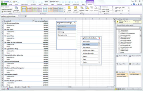
In the dialog box, click “New Worksheet,” and then OK. In the new worksheet, the “PivotTable Fields” tab on the right side of the screen should now be visible. You may now start dragging the fields to the following areas: filters, columns, rows, or values, with the ultimate goal of adjusting the way the data is presented in accordance with your preferred method and visual format.
Conditional Formatting
This feature operates using logic and allows you to apply specific formatting to cells that meet certain preset criteria. For instance, you may want to highlight cells which present values less than 100.
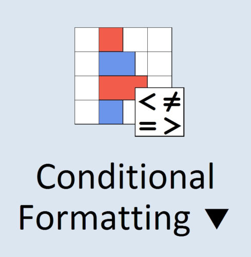
From the “Home” tab, click “Conditional Formatting,” and then in “Highlight Cells Rules,” choose “Less than.” Specify the value (100) in the dialog box, as well as your preferred color of the highlighted cell, and then click OK. This way, all figures which go below 100 will be highlighted. Other conditional formatting options are also available such as data bars and color scales.
Index–Match
Index–Match is similar to the VLOOKUP feature which allows you to easily find the data you’re looking for, only that it is a combination of two functions—Index and Match. By simply typing in the word “INDEX” in the formula, selecting the range of cells from which you want to look up the data, then indicating its numeric position in the list, you will be able to retrieve the name of the information you’re looking for.
“MATCH” appears to be the opposite because here you indicate the name of the information, and Excel will give you the numeric position of the item in the list.
Macros And VBA
Macros let you automate tasks after clicking a button. Turn to the “Developer” tab, click “Customize the Ribbon,” and once the dialog box pops up, check “Developer” and then OK. Back in the “Developer” tab, choose a command button that would trigger the automation, such as “Start.” Right click on “Start,” and choose “View Code.”
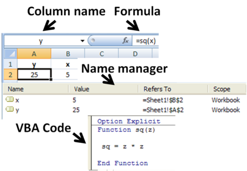
On the Visual Basic Editor dialog box that would appear, add the data that you wish to appear after clicking on the “Start” button. With that, with just one click of the command button, you can generate automated results.
These ingenious features of Microsoft Excel that are simply waiting in the corners for you to discover. So take the time to explore them one by one and keep practicing for you to be able to harness its full potential for your benefit in the workplace.